6 Analysis of variance, calculation and expression of precision estimates
6.1 General
After the data have been inspected for uniformity, a transformation has been performed if necessary, and any outliers have been rejected (see Clause 5), an analysis shall be carried out. First an analysis-of-variance table shall be constructed, and finally the precision estimates derived.
6.2 Analysis of variance
6.2.1 Forming the sums of squares for the laboratories x samples interaction sum of squares
6.2.1.1 General
The estimated values, if any, shall be put in the array and an approximate analysis of variance performed.
Mean correction, Mc = T2/2L'S'
where L' is L minus the number of laboratories rejected in 5.6 minus the number of laboratories with no remaining results after rejections in 5.3.3.

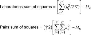
The laboratories x samples interaction sum of squares, I, is given by:
I = (pairs sum of squares) − (laboratories sum of squares) − (sample sum of squares)
Ignoring any pairs in which there are estimated values,

The purpose of performing this approximate analysis of variance is to obtain the minimized laboratories x samples interaction sum of squares, I. This is then used as indicated in 6.2.2, to obtain the laboratories sum of squares.
If there were no estimated values, the above analysis of variance is exact and 6.2.2 shall be disregarded.
6.2.1.2 Worked example
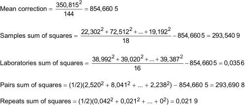
Table 8 can then be derived.
6.2.2 Forming the sum of squares for the exact analysis of variance
6.2.2.1 General
In 6.2.2, all the estimated pairs are disregarded and new values of gj are calculated. The following sums of squares for the exact analysis of variance are formed.
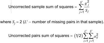
The laboratories sum of squares is equal to (pairs sum of squares) − (samples sum of squares) − (the minimized laboratories x samples interaction sum of squares)

6.2.2.2 Worked example

6.2.3 Degrees of freedom
6.2.3.1 General
The degrees of freedom for the laboratories are (L' − 1). The degrees of freedom for laboratories x samples interaction are (L' − 1)(S' − 1) for a complete array and are reduced by one for each pair which is estimated. The degrees of freedom for repeats are (L'S') and are reduced by one for each pair in which one or both values are estimated.
6.2.3.2 Worked example
There are eight samples and nine laboratories in this example. As no complete laboratories or samples were rejected, then S' = 8 and L' = 9.
Laboratories degrees of freedom = L' − 1 = 8
Laboratories x samples interaction degrees of freedom, if there had been no estimates, would have been (9 − 1)(8 − 1) = 56. But one pair was estimated, hence laboratories x samples interaction degrees of freedom = 55. Repeats degrees of freedom would have been 72 if there had been no estimates. In this case, one pair was estimated, hence repeats degrees of freedom = 71.
6.2.4 Mean squares and analysis of variance
6.2.4.1 General
The mean square in each case is the sum of squares divided by the degrees of freedom. This leads to the analysis of variance shown in Table 9.
The ratio ML/MLS is distributed as F with the corresponding laboratories and interaction degrees of freedom (see Clause C.7). If this ratio exceeds the 5 % critical value given in Table D.6, then bias between the laboratories is implied and the programme organizer shall be informed (see 4.5): further standardization of the test method can be necessary.
6.2.4.2 Worked example
The analysis of variance is shown in Table 10.
The ratio ML/MLS = 0.0044/0.002078 has a value 2.117. This is greater than the 5 % critical value obtained from Table D.6, indicating bias between laboratories.
6.3.1 Expectation of mean squares with no estimated values
For a complete array with no estimated values, the expectations of mean squares are:

6.3.2 Expectation of mean squares with estimated values
6.3.2.1 General
The coefficients of σ0(2) and σ2(2) in the expectation of mean squares are altered in the cases where there are estimated values. The expectations of mean squares then become:

where
β = 2[(K - S')/(L' - 1)]
K is the number of laboratory x sample cells containing at least one result;
α and γ are computed as follows.
If there are no cells with only a single estimated result, then α = γ = 1.
If there are no empty cells (i.e. every laboratory has tested every sample at least once, and K = L' x S'), then α and γ are both 1 plus the proportion of cells with only a single result.
If there are both empty cells and cells with only one result, then for each laboratory compute the proportion, pi, of samples tested for which there is only one result, and the sum, P, of these proportions over all laboratories. For each sample, compute the proportion, qj, of laboratories that have tested the sample for which there is only one result, and the sum, Q, of these proportions over all samples. Compute the total number of cells, W, with only one result and the proportion of these among all non-empty cells, W/K. Then:
α = 1 + [(P - (W/K))/(L' - 1)]
and
γ = 1 + [(W - P - Q +(W/K))/(K - L' - S' + 1)]
NOTE The development in 6.3.2 is based upon the assumption that both samples and laboratories are "random effects".
6.3.2.2 Worked example
For the example that has eight samples and nine laboratories, one cell is empty (laboratory D for sample 1), so K = 71 and

None of the non-empty cells has a single result, so α = γ = 1.
6.3.3 Calculation of precision estimates
6.3.3.1 Repeatability
The repeatability variance is twice the mean square for repeats. The repeatability estimate is the product of the repeatability standard deviation and the "t-value", tv, with appropriate degrees of freedom, v (see Table D.5), corresponding to a two-sided probability of 95 %.
This calculated estimate shall be rounded to no fewer than three and no more than four significant digits.
Note that if a transformation Y = F(x) has been used, then

where r(x), r(y) are the corresponding repeatability functions (see Table E.1). A similar relationship applies to the reproducibility functions R(x), R(y).
6.3.3.2 Worked example

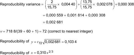
6.3.3.3 Reproducibility
The reproducibility variance, VR, is expressed as

where the symbols are as set out in 6.2.4 and 6.3.2.
The reproducibility estimate is the product of the reproducibility standard deviation and the "t-value", tv, with appropriate degrees of freedom, v, (see Table D.5), corresponding to a two-sided probability of 95 %. An approximation to the degrees of freedom of the reproducibility variance is given by Equation (15).

where
r1, r 2 and r 3 are the three successive terms in Equation (14);
vLS is the degrees of freedom for laboratories x samples;
vr is the degrees of freedom for repeats.
The calculated estimate of reproducibility shall also be rounded to no fewer than three and no more than four significant digits.
Substantial bias between laboratories results in a loss of degrees of freedom estimated by Equation (15). If reproducibility degrees of freedom are less than 30, then the programme organizer shall be informed (see 4.5); further standardization of the test method can be necessary.
6.3.3.4 Worked example
6.4 Expression of precision estimates of a method of test
6.4.1 When the precision of a method of test has been determined in accordance with the procedures set out in this International Standard, it shall be included in the method as follows:
"X Precision
X.1 General
The precision, as determined by statistical examination in accordance with ISO 4259 of inter-laboratory test results on (type of products) with test results in the range (x to y), is given in X.2 and X.3.
X.2 Repeatability
The difference between two test results obtained by the same operator with the same apparatus under constant operating conditions on identical test material would, in the long run, in the normal and correct operation of the test method, exceed the following value (value given in Table M)(value shown in Figure N) in only one case in twenty:
r = fr(x)
where x is the average of the test results being compared.
X.3 Reproducibility
The difference between two single and independent test results obtained by different operators working in different laboratories on identical test material would, in the long run, in the normal and correct operation of the test method, exceed the following value (value given in Table M) (value shown in Figure N) in only one case in twenty:
R = fR(x)
where x is the average of the test results being compared.
6.4.2 Only in exceptional cases shall a precision estimate not based upon ISO 4259 be allowed. In those cases, the alternative introductory text below shall be used:
"The precision evaluation programme for the matrix of samples with (p) contents in the range (q to r) did not conform to the requirements of ISO 4259, and thus only an estimate of precision based upon inter-laboratory test results is given in X.2 and X.3."
6.4.3 The size of the matrix of samples used to generate the precision statement shall not be quoted unless it is for the reason given in 6.4.2 that has been exercised.
