ASTM D6300 Standard Practice for Determination of Precision and Bias Data for Use in Test Methods for Petroleum Products and Lubricants
8. Analysis of Variance and Calculation of Precision Estimates
8.1 After the data have been inspected for uniformity, a transformation has been performed, if necessary, and any outliers have been rejected (see Section 7), an analysis of variance shall be carried out. First an analysis of variance table shall be constructed, and finally the precision estimates derived.
8.2 Analysis of Variance:
8.2.1 Forming the Sums of Squares for the Laboratories x Samples Interaction Sum of Squares - The estimated values, if any, shall be put in the array and an approximate analysis of variance performed.

where:
L' = L - number of laboratories rejected in 7.6-number of laboratories with no remaining results after rejections in 7.3.4,
S' = total of remaining pairs in the jth sample, and
T = the total of all duplicate test results.
Samples sum of squares =

where gj is the sum of sample j test results.
Laboratories sum of squares =

where hi is the sum of laboratory i test results.
Pairs sum of squares =

I = Laboratories x samples interaction sum of squares = (pairs sum of squares) - (laboratories sum of squares) - (sample sum of squares)
Ignoring any pairs in which there are estimated values, repeats sum of squares,

The purpose of performing this approximate analysis of variance is to obtain the minimized laboratories x samples interaction sum of squares, I. This is then used as indicated in 8.2.2, to obtain the laboratories sum of squares. If there were no estimated values, the above analysis of variance is exact and paragraph 8.2.2 shall be disregarded.
8.2.1.1 Worked Example:
Mean correction =
 = 854.6605
where 854.6605 is the result obtained by electronic calculation without rounding the factors in the expression.
Samples sum of squares

Laboratories sum of squares

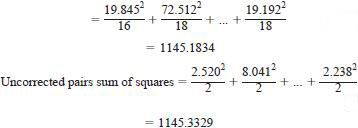
Pairs sum of squares
 = 293.6908
Repeats sum of squares =
 = 0.0219
Table 10 can then be derived.
8.2.2 Forming the Sum of Squares for the Exact Analysis of Variance:
8.2.2.1 In this subsection, all the estimated pairs are disregarded and new values of gj are calculated. The following sums of squares for the exact analysis of variance (8) are formed.

where:
Sj = 2(L' - number of missing pairs in that sample).

The laboratories sum of squares is equal to (pairs sum of squares) - (samples sum of squares) - (the minimized laboratories 3 samples interaction sum of squares)

8.2.2.2 Worked Example:
Uncorrected samples sum of squares

Therefore, laboratories sum of squares

8.2.3 Degrees of Freedom:
8.2.3.1 The degrees of freedom for the laboratories are (L' - 1). The degrees of freedom for laboratories x samples interaction are (L' - 1)(S' - 1) for a complete array and are reduced by one for each pair which is estimated. The degrees of freedom for repeats are (L'S') and are reduced by one for each pair in which one or both values are estimated.
8.2.3.2 Worked Example - There are eight samples and nine
laboratories in this example. As no complete laboratories or
samples were rejected, then S' = 8 and L' = 9.
Laboratories degrees of freedom = L-1 = 8.
Laboratories x samples interaction degrees of freedom if there had been no estimates, would have been (9–1)(8–1) = 56. But one pair was estimated, hence laboratories 3 samples interaction degrees of freedom = 55. Repeats degrees of freedom would have been 72 if there had been no estimates. In this case one pair was estimated, hence repeats degrees of freedom = 71.
8.2.4 Mean Squares and Analysis of Variance:
8.2.4.1 The mean square in each case is the sum of squares divided by the corresponding degrees of freedom. This leads to the analysis of variance shown in Table 11. The ratio ML/MLS is distributed as F with the corresponding laboratories and interaction degrees of freedom (see A1.7). If this ratio exceeds the 5 % critical value given in Table A2.6, then serious bias between the laboratories is implied and the program organizer shall be informed (see 6.5); further standardization of the test method may be necessary, for example, by using a certified reference material.
8.2.4.2 Worked Example - The analysis of variance is shown in Table 12. The ratio ML/MLS 5 0.0044/0.002078 has a value 2.117. This is greater than the 5 % critical value obtained from Table A2.6, indicating bias between laboratories.
8.3 Expectation of Mean Squares and Calculation of Precision Estimates:
8.3.1 Expectation of Mean Squares with No Estimated Values-For a complete array with no estimated values, the expectations of mean squares are

where:
 = the component of variance due to interaction between laboratories and samples, and
 = the component of variance due to differences between laboratories.
8.3.2 Expectation of Mean Squares with Estimated Values:
8.3.2.1 The coefficients of and in the expectation of mean squares are altered in the cases where there are estimated values. The expectations of mean squares then become


where:
K = the number of laboratory x sample cells containing at least one result, and a and g are computed as in 8.3.2.5
8.3.2.2 If there are no cells with only a single estimated result, then α = γ = 1.
8.3.2.3 If there are no empty cells (that is, every lab has tested every sample at least once, and K = L' x S'), then a and g are both one plus the proportion of cells with only a single result.
8.3.2.4 If there are both empty cells and cells with only one result, then, for each lab, compute the proportion of samples tested for which there is only one result, pi, and the sum of these proportions over all labs, P. For each sample, compute the proportion of labs that have tested the sample for which there is only one result on it, qj, and the sum of these proportions over samples, Q. Compute the total number of cells with only one result, W, and the proportion of these among all nonempty cells, W/K. Then

NOTE 5 - These subsections are based upon the assumptions that both samples and laboratories are random effects.
8.3.2.5 Worked Example - For the example, which has eight samples and nine laboratories, one cell is empty (Laboratory D on Sample 1), so K = 71 and

None of the nonempty cells has only one result, so α = γ = 1. To make the example more interesting, assume that only one result remains from Laboratory A on Sample 1. Then W = 1, p1 = 1/8, p2 = p3 = ... = p9 = 0, and P = 0.125. We compute q1 = 1/8 (we don't count Laboratory D in the denominator), q2 = q3 =...= q8 = 0, and Q = 0.125. Consequently,

8.3.3 Calculation of Precision Estimates:
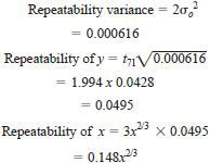
8.3.3.1 Repeatability - The repeatability variance is twice the mean square for repeats. The repeatability estimate is the product of the repeatability standard deviation and the "t-value" with appropriate degrees of freedom (see Table A2.5) corresponding to a two-sided probability of 95 %. Round calculated estimates of repeatability in accordance with Practice E 29, specifically paragraph 7.6 of that practice. Note that if a transformation y 5 f(x) has been used, then

where r(x), r(y) are the corresponding repeatability functions (see Table A3.1). A similar relationship applies to the reproducibility functions R(x), R(y).
8.3.3.2 Worked Example:


Reproducibility variance

where the symbols are as set out in 8.2.4 and 8.3.2. The reproducibility estimate is the product of the reproducibility standard deviation and the "t-value" with appropriate degrees of freedom (see Table A2.5), corresponding to a two-sided probability of 95 %. An approximation (9) to the degrees of freedom of the reproducibility variance is given by Eq 39.

where:
r1, r 2, and r3 = the three successive terms in Eq 38,
vLS = the degrees of freedom for laboratories x samples, and
vr = the degrees of freedom for repeats.
(a) Round calculated estimates of reproducibility in accordance with Practice E 29, specifically paragraph 7.6 of that practice.
(b) Substantial bias between laboratories will result in a loss of degrees of freedom estimated by Eq 39. If reproducibility degrees of freedom are less than 30, then the program organizer shall be informed (see 6.5); further standardization of the test method may be necessary.
8.3.3.4 Worked Example - Recalling that α = γ = 1 (not 1.014, as shown in Eq 34 and 35):
Reproducibility variance


8.3.3.5 Determinability - When determinability is relevant, it shall be calculated by the same procedure as is used to calculate repeatability except that pairs of determined values replace test results. This will as much as double the number of "laboratories" for the purposes of this calculation.
8.3.4 Bias:
8.3.4.1 Bias equals average sample test result minus its accepted reference value. In the ideal case, average 30 or more test results, measured independently by processes in a state of statistical control, for each of several relatively uniform materials, the reference values for which have been established by one of the following alternatives, and subtract the reference values. In practice, the bias of the test method, for a specific material, may be calculated by comparing the sample average with the accepted reference value.
8.3.4.2 Accepted reference values may be one of the following: an assigned value for a Standard Reference Material, a consensus value based on collaborative experimental work under the guidance of a scientific or engineering organization, an agreed upon value obtained using an accepted reference method, or a theoretical value.
8.3.4.3 Where possible, one or more materials with accepted reference values shall be included in the interlaboratory program. In this way sample averages free of outliers will become available for use in determining bias.
8.3.4.4 Because there will always be at least some bias because of the inherent variability of test results, it is recommended to test the bias value by applying Student's t test using the number of laboratories degrees of freedom for the sample made available during the calculation of precision. When the calculated t is less than the critical value at the 5 % confidence level, the bias should be reported as not significant.
8.4 Precision and Bias Section for a Test Method - When the precision of a test method has been determined, in accordance with the procedures set out in this practice, it shall be included in the test method as illustrated in these examples:
8.4.1 Precision - The precision of this test method, which was determined by statistical examination of interlaboratory results using Practice D6300, is as follows.
8.4.1.1 Repeatability - The difference between successive results obtained by the same operator with the same apparatus under constant operating conditions on identical test material would in the long run, in the normal and correct operation of the test method exceed the following values only in one case in 20.

where x is the average of two results.
8.4.1.2 Reproducibility - The difference between two single and independent results obtained by different operators working in different laboratories on identical test material would in the long run exceed the following values only in one case in 20.

where x is the average of two results.
8.4.1.3 If determinability is relevant, it shall precede repeatability in the statement above. The unit of measurement shall be specified when it differs from that of the test result:
8.4.1.4 Determinability - The difference between the pair of determined values averaged to obtain a test result would, in the long run, in the normal and correct operation of the test method, exceed the following value in only one case in 20. When this occurs, the operator must take corrective action:

where m is the mean of the two determined values in mL.
8.4.2 A graph or table may be used instead of, or in addition to, the equation format shown above. In any event, it is helpful to include a table of typical values like Table 13.
8.4.3 The wording to be used for test methods where the statistical treatment applied is unknown is: "The precision of this test is not known to have been obtained in accordance with currently accepted guidelines (for example, in Committee D-2, Practice D6300)". The existing statement of precision would then follow.
8.5 Data Storage:
8.5.1 The interlaboratory program data should be preserved for general reference. Prepare a research report containing details of the test program, including description of the samples, the raw data, and the calculations described herein. Send the file to ASTM Headquarters and request a File Reference Number.
8.5.2 Use the following footnote style in the precision section of the test method. "The results of the cooperative test program, from which these values have been derived, are filed at ASTM Headquarters as RR:D02: XXXX".
9. Keywords
9.1 interlaboratory; precision; repeatability; reproducibility; round robin

